Cluster-Outlier Analysis
Studio applies Anselin's Local Indicators of Spatial Association (LISA), specifically the local Moran statistic, to identify geographical clusters of values or find geographical outliers.
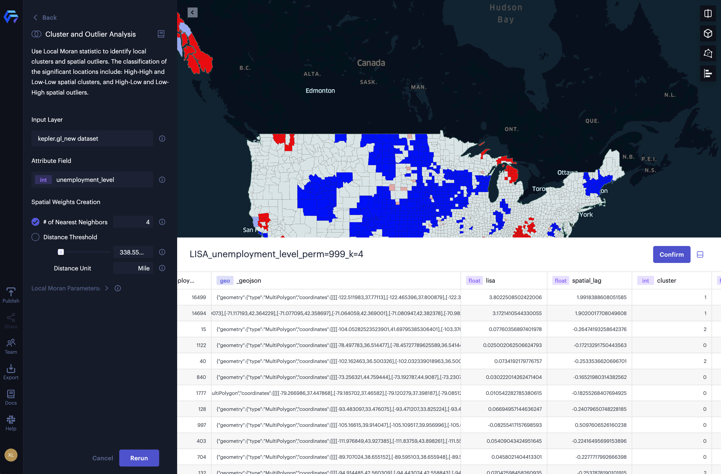
An example of cluster and outlier analysis.
This method has been widely used in spatial application fields including environmental and natural resource analysis, real estate analysis, criminology studies, public health research, political geography and demographics studies, and much more.
Cluster and Outlier Analysis helps answer questions such as:
- Which US counties have high caseloads of Covid-19?
- Are there spatial patterns in the listing price of Airbnb rentals in the city?
- Are there any restaurants with significantly more/fewer visits than nearby competitors?
Cluster Types
The local Moran statistic takes the data values and the associated geographical locations as input, then returns statistically significant clusters in which values are concentrated in two different forms.
The below chart describes the four cluster types found in the local Moran statistic:
| Cluster | Description |
|---|---|
| High-High | Hot spot clusters containing high values surrounded by other high values. |
| Low-Low | Cold spot clusters containing low values surrounded by other low values. |
| High-Low | Spatial outlier where high values are surrounded by low values. |
| Low-High | Spatial outlier where low values are surrounded by high values. |
Performing a Cluster and Outlier Analysis
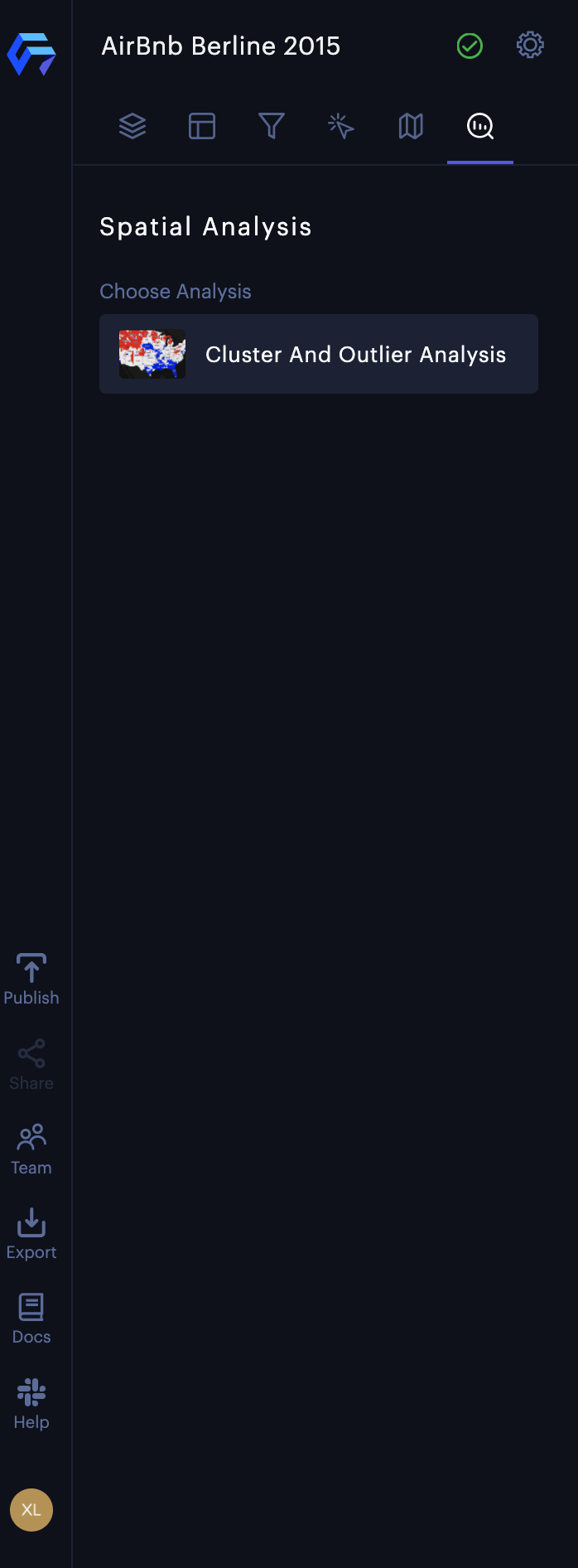
Navigate to the Analysis tab in Studio, then click Cluster And Outlier Analysis button. (See figure 2: left)
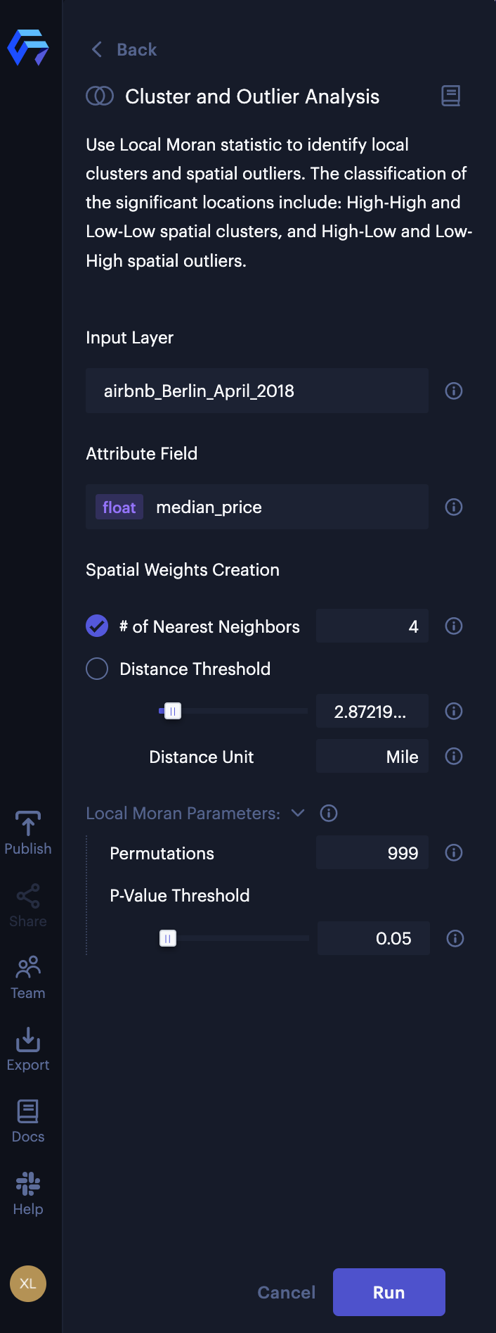
Once you click the button, a side panel appears with configuration options for the "Cluster and Outlier Analysis" feature. (See Figure 2: right)
 |  |
Configuration of Cluster and Outlier Analysis
The Cluster and Outlier Analysis contains four sections:
- Input layer: select the layer you will apply cluster and outlier analysis.
- Attribute Field: select the attribute field from the input layer.
- Spatial Weights Creation: choose one of the two types of spatial weights to define geographical neighboring structure: 1) k-nearest neighbors and 2) distance threshold-based spatial weights.
- Local Moran Parameters: change the parameters for local moran statistic.
Input Layer
Studio supports cluster and outlier analysis on the layer with either points or polygons geometries.
In the Input Layer section, you can select a Point Layer, or a GeoJson Layer with Point or Polygon geometries.
Attribute Field
In the Attribute Field section, select a numerical field that you want to apply cluster and outlier analysis.
Note: For local Moran statistics, we suggest selecting a quantitative variable. Studio will support more LISA methods for binary variables, bivariate, and multivariate variables. Please contact us for more information.
Spatial Weights Creation
In the Spatial Weights Creation section, Studio provides two different types of distance-based spatial weights:
- K nearest neighbors-based weights.
- Distance threshold-based weights.
Geometries in the input layer will be used to create spatial weights that represent the geographical neighboring structure.
Note: Studio will support more spatial weights creation methods. Please contact us for more information.

The options of spatial weights creation.
K Nearest Neighbors Based Weights
You can check the # of Nearest Neighbors option and input the number of nearest neighbors, which ensures that all spatial objects have the same number of neighbors.
Distance Threshold Based Weights
You can check the Distance Threshold option and input the value of distance thresholds or bands to define the neighbors for each spatial object as those falling within a threshold distance.
You can choose the distance unit to be either "Mile" or "KM" (kilometer). The Studio suggests a distance threshold value that guarantees every spatial object has at least one neighbor. However, you should always adjust the threshold value based on the use case, avoiding expensive computation and memory usage.
Local Moran Parameters
In local Moran statistics, the permutation-based inference is used to test the statistical significance of each cluster. The result is a pseudo p-value that can be used to assess the significance of each cluster.
You can control the following parameters for permutation-based inference:
- Permutations
You can input the value for the number (e.g. 999) of Permutations to generate 999 randomly-shuffled neighboring values for each spatial object. The local Moran's I value of each spatial object is then tested against the 999 local Moran's I values with randomly-composed neighbors to evaluate if the cluster values are "significantly" spatial autocorrelated.

The local Moran parameters.
- P-Value Threshold
With the pseudo p-values for each spatial object, you can define the P-Value Threshold to only display significant clusters at a certain level on the map. The default p-value threshold is 0.05 with 999 permutations. It is a good practice to assess the sensitivity of the significant clusters to the number of permutations.
Note: in permutation-based inference, the smallest pseudo p-value is computed as
1/(permutations + 1). For example, the smallest pseudo p-value is 0.001 for 999 permutations.
Results
The results will be stored in a new dataset which you can preview in a data table (see Figure below 5). It includes several columns:
| Column Name | Description |
|---|---|
| Attribute Field | The value of selected Attribute Field. |
| latitude (optional) | The latitude value (only when Input Layer is a Point layer). |
| longitude (optional) | The longitude value, only when Input Layer is a Point layer |
| lisa | The local Moran's I value. |
| spatial_lag | The average (standardized) value of the neighbors. |
| cluster | The type of spatial association - 0 for not significant, 1 for High-High, 2 for Low-Low, 3 for High-Low, 4 for Low-High, 5 for isolated (no neighbors). |
| pvalue | The pseudo p-value is the significance value computed from the random permutations. |
| neighbors | The array of row indices of the neighbors. |
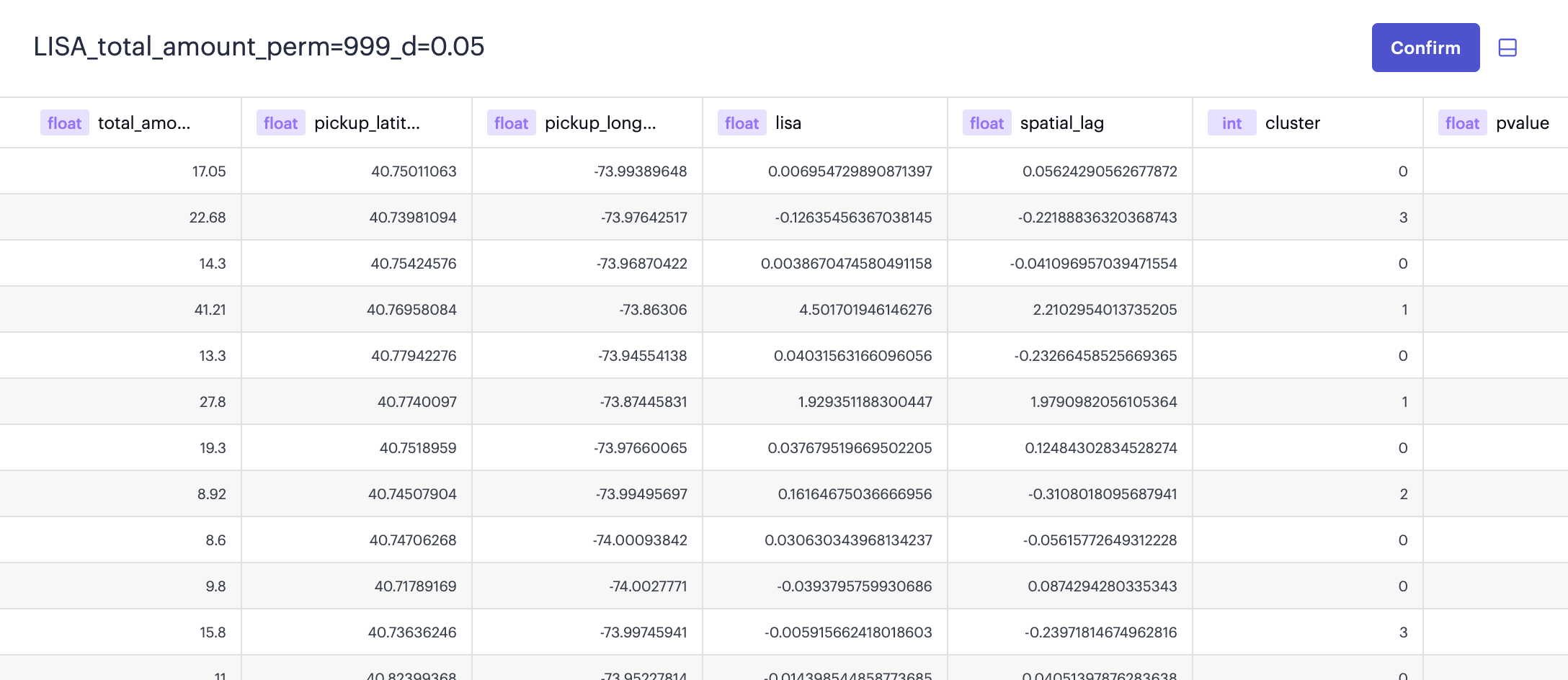
The preview of the result table.
Once you click Confirm, a new dataset and a new layer of the LISA results will be created. If the input layer is a Point layer, a Connectivity Graph layer will generate to visualize the neighboring/connectivity relationship among the spatial objects (see Figure below). You can mouse over a point to highlight its neighboring points that are defined by the spatial weights option.
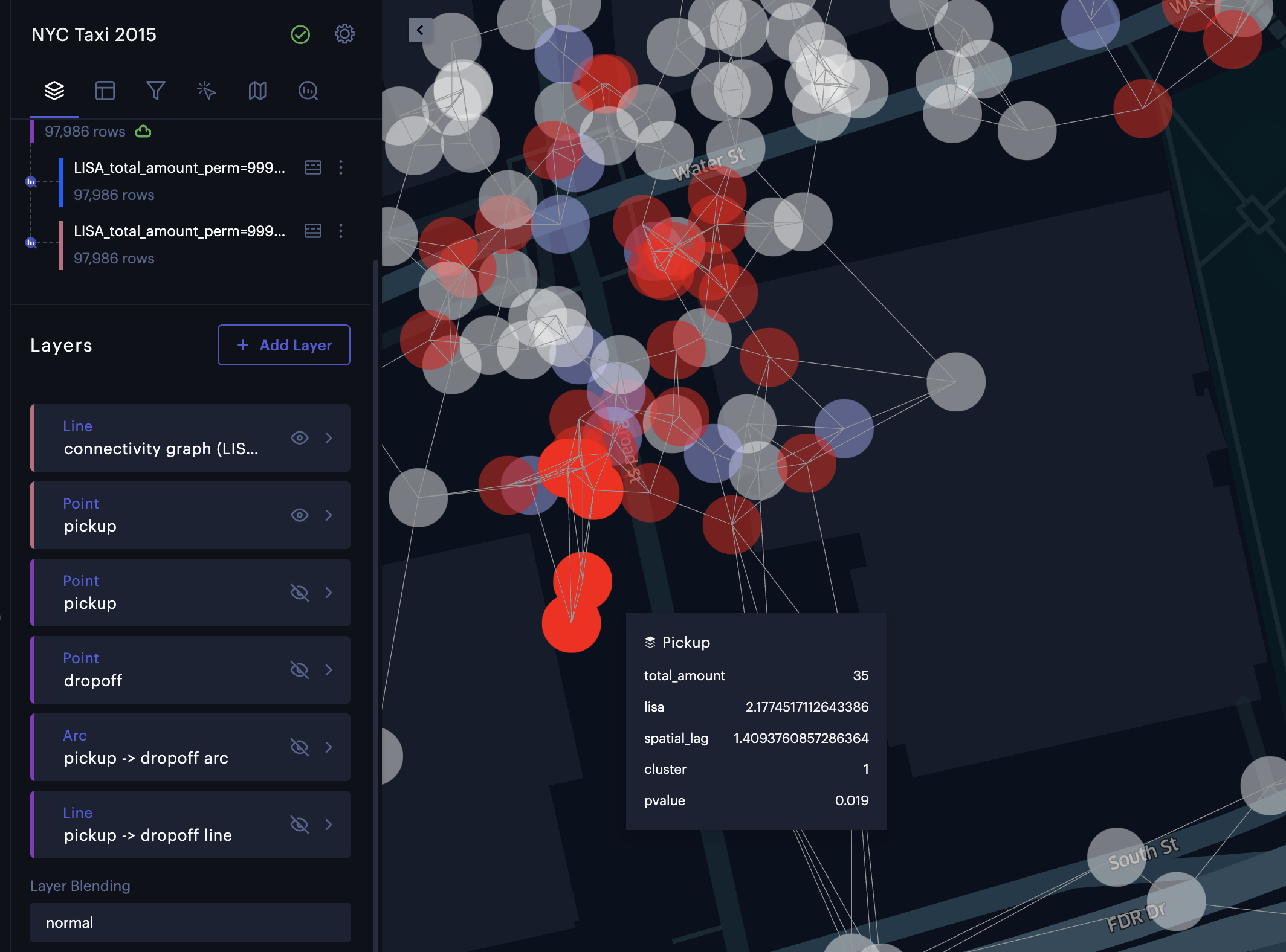
The connectivity graph layer created from the Point layer.
Cluster and Outlier Analysis Example
1. NYC Taxi Trips
The NYC taxi trip data include 97,985 trips in New York City. Using cluster and outlier analysis, we can explore the spatial distribution of taxi fees, finding which pick-up and drop-off locations often have the highest-paying passengers.
1. Click Analysis icon, then click Cluster and Outlier.
2. Select the input layer. In this case, pickup from the dataset nyc_taxi.csv.
3. Select the attribute field. In this case total_amount.
4. Select Distance Threshold, the input 0.05 and select KM. This allows us to compare the taxi fee for each pick-up location with other pick-up locations within 50 meters.
5. To better illustrate significant clusters, set the P-Value Threshold to 0.001.
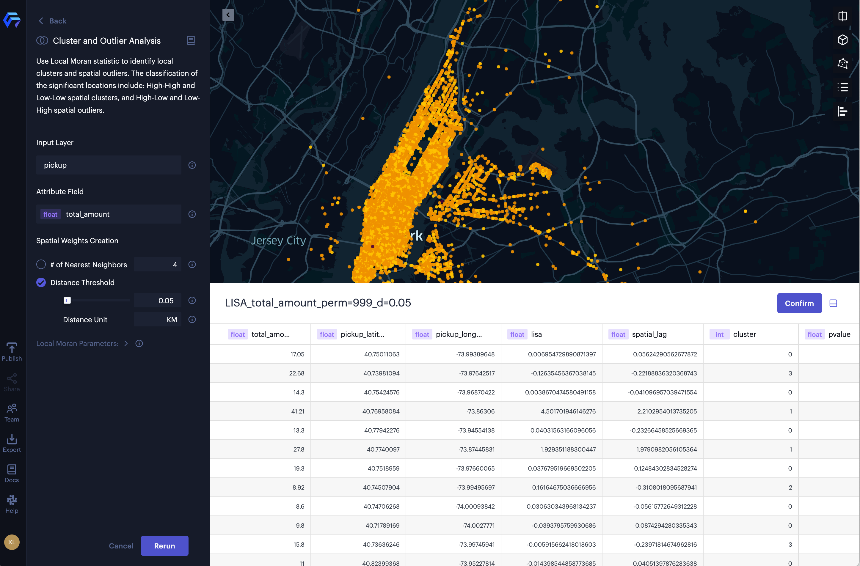
Cluster and outlier analysis of taxi fee (total amount) in New York.
The result of the cluster and outlier analysis is a new dataset and two new layers showing the 4 different types of clusters and the connectivity graph. To better illustrate the hot and cold spots, we hide the spatial outliers (see Figure below). From the results, we can observe hot spots of high taxi fees in the lower Manhattan area, midtown Manhattan area, the LaGuardia airport, and JFK airport. The cold spots of low taxi fees can be discovered in the midtown Manhattan area (especially the east side of central park).
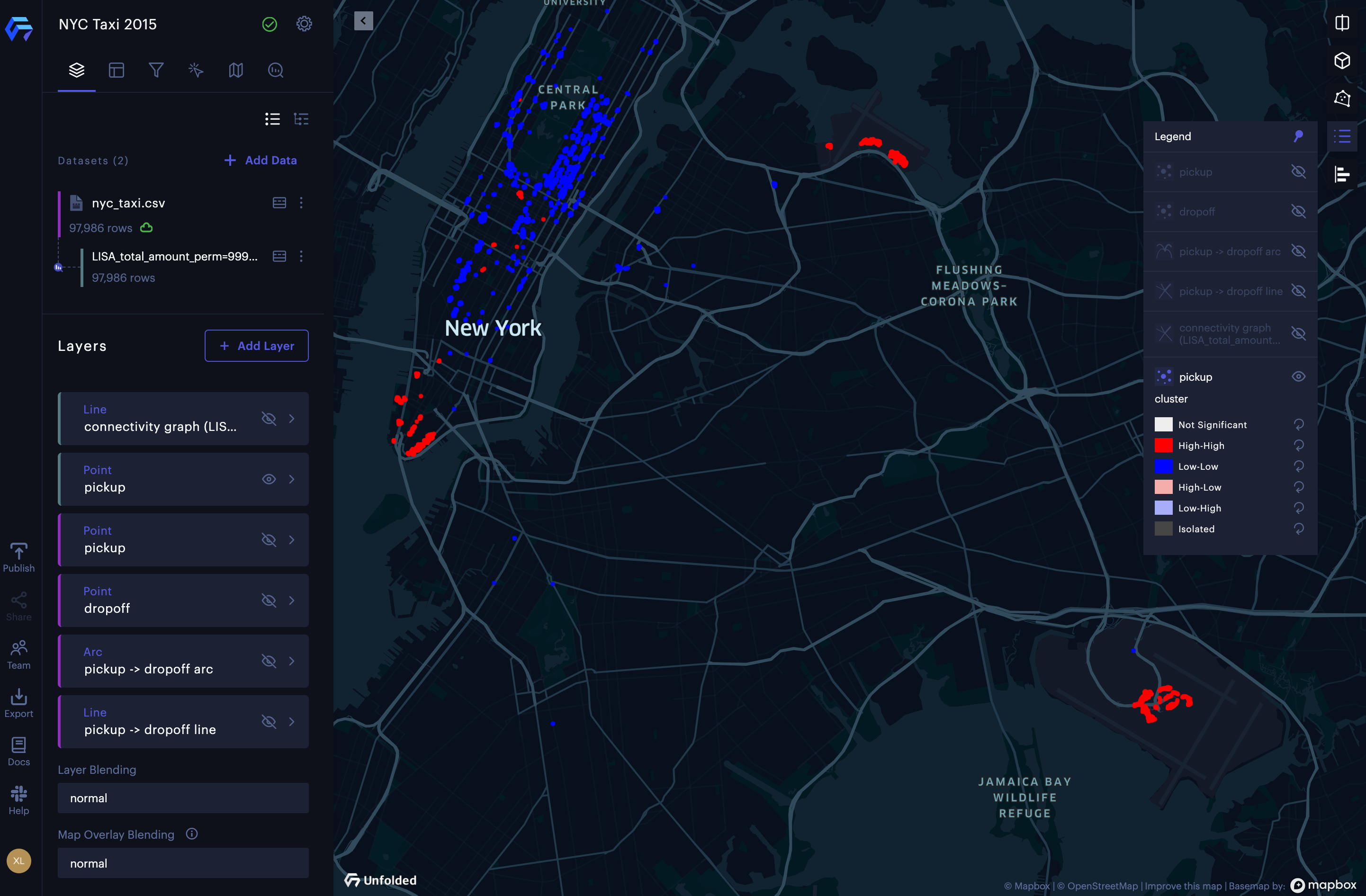
The result of cluster and outlier analysis of taxi fees (total amount) in New York.
2. Airbnb Rents in Berlin
In this example, we are going to analyze the spatial pattern of the median listing price of Airbnb rentals in 138 districts in Berlin. The data is available to download at GeoPython 2018 workshop. We can use Studio to explore if there are any hot spots of the Airbnb median listing price in Berlin.
1. Click Analysis icon, then click Cluster and Outlier.
2. Select the input layer. In this case, airbnb_Berlin_April_2018.geojson.
3. Select the attribute field. In this case median_price.
4. Select # of Nearest Neighbors, then input 4 for the spatial weights creation.
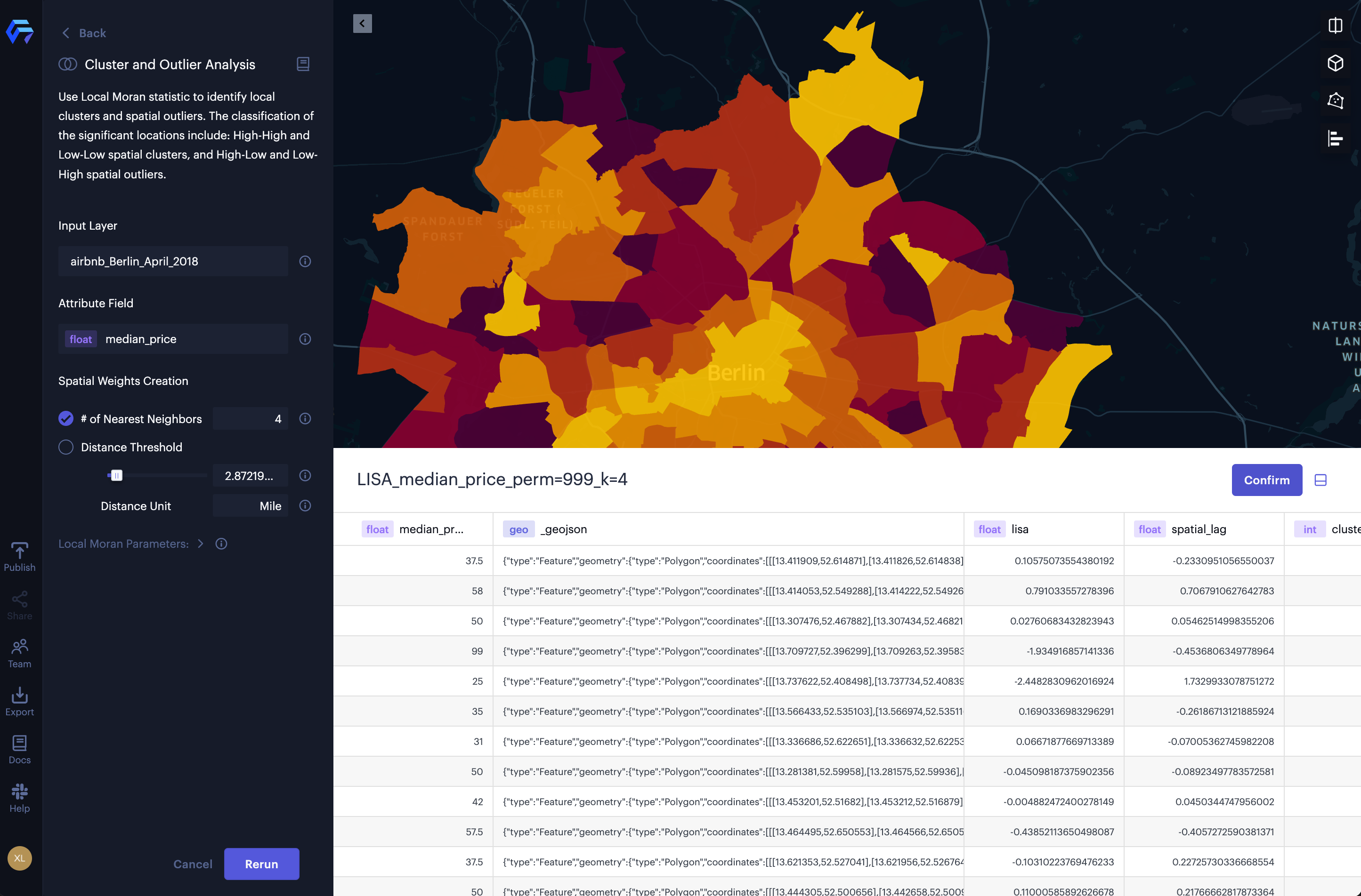
Cluster and outlier analysis of the median listing price of Airbnb rentals in Berlin.
The results of the cluster and outlier analysis are a new dataset and a new layer showing the 4 different types of clusters. From the results, we can observe hot spots (High-High clusters) of median listing prices in the central Berlin area (around Mitte), and cold spots (Low-Low clusters) of median listing prices in the northern Berlin area (around Reinickendorf, a residential area). There is also a significant High-Low cluster (a spatial outlier where high listing prices are surrounded by low listing prices), which is near the Wannsee scenic area, in the southwest of Berlin. The spatial outliers and cold spots can be observed in the southeast of Berlin (near Treptow-Köpenick), which is an area mixed with historical attractions, old industrial areas, and natural attractions.
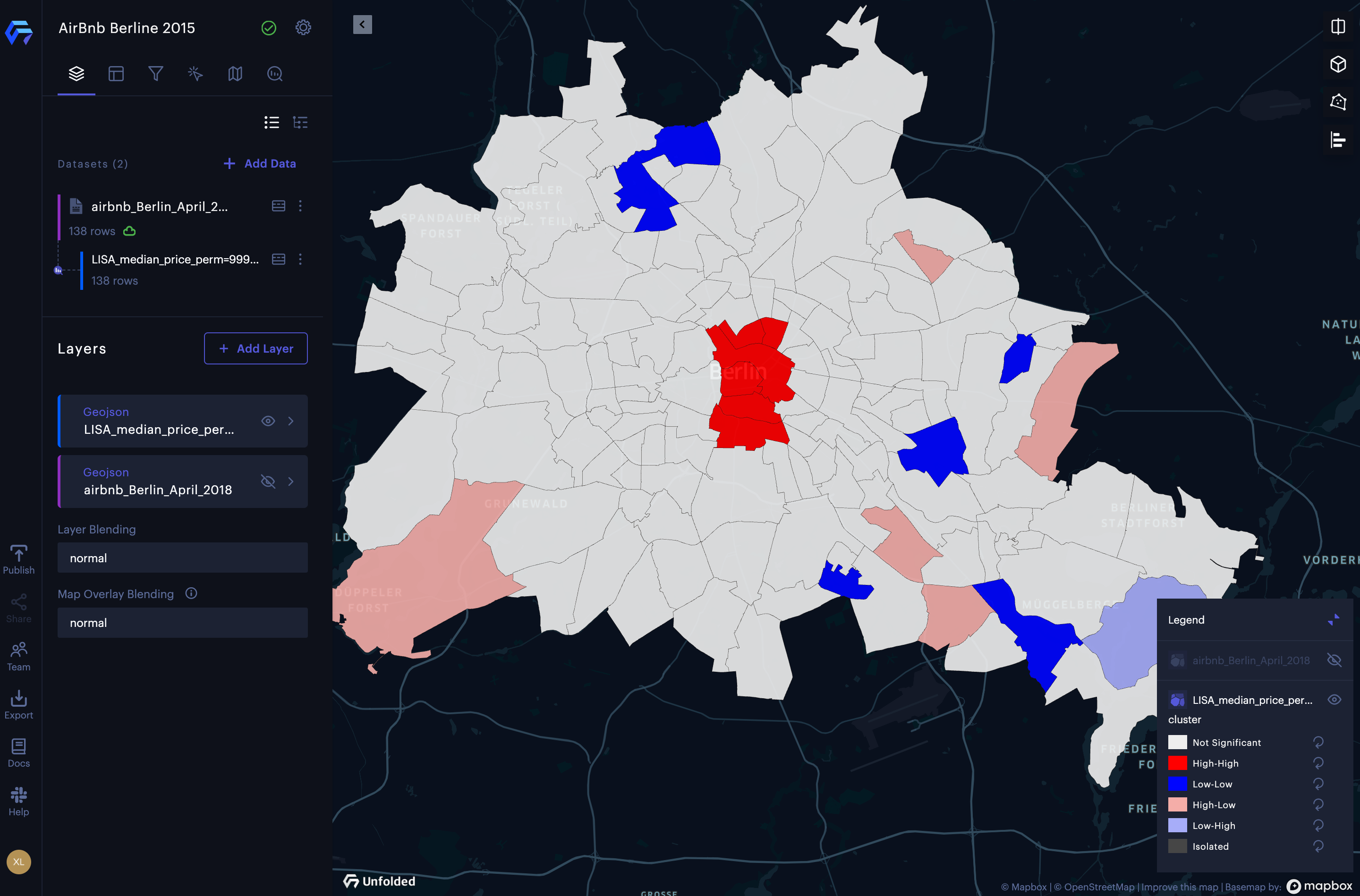
The result of cluster and outlier analysis of the median listing price of Airbnb rentals in Berlin.
Updated 3 months ago
