
Spatial Desktop
FSQ Spatial Desktop is our offering designed for tech-savvy GIS professionals seeking advanced desktop computing capabilities. It leverages Kepler.gl's visualization excellence with native DuckDB to overcome browser limitations, allowing for powerful spatial analysis and compelling visualizations of multi-gigabyte datasets without memory bottlenecks or cloud dependencies. The product is built on the open-source SQLRooms framework, promoting community-driven extensibility through plugins, and provides complete analytical capability without internet connectivity requirements.
Key Components
- Projects: A "Project" refers to a collection of your work, including the datasets you're using, the queries you've run, and the visualizations you've created.FSQ Spatial Desktop provides the capability to manage multiple projects and save them locally to your desktop or your FSQ Cloud storage
- Data Sources Panel: This is the central hub for managing your datasets, including tables and tilesets, allowing you to easily access and integrate various spatial data formats.
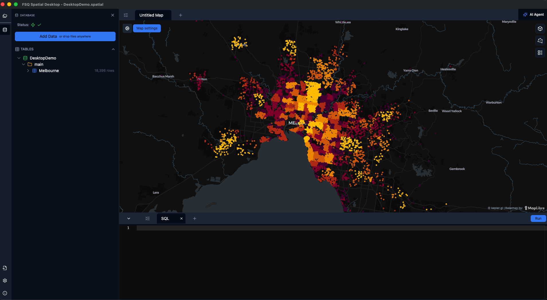
- Map View (Powered by Kepler.gl): A dedicated visualization canvas for geographical data, enabling real-time rendering of millions of data points, heatmaps, clusters, and interactive filtering. Toggle and modify using the Layers icon.
- SQL Query Editor (Leveraging DuckDB): An interactive environment where you can write and execute SQL queries for complex spatial analysis, benefiting from DuckDB's sub-second query performance on large datasets.
- Spatial Agent: Use an advanced AI agent to create datasets, generate insights, access H3 Hub data, and perform full analysis from start to finish
All the components of FSQ Spatial Desktop are built on top of the SQL Rooms Framework.
Download and Install
Steps:
- Open your web browser and navigate to the FSQ Spatial Desktop download page
- On the download page, choose the appropriate version for your operation system.
macOS (13 Ventura or later):
- Choose the appropriate version for your Mac: Apple Silicon (FSQ-Spatial-version-arm64.dmg) or Intel (FSQ-Spatial-version-x64.dmg).
- Save the installer file (e.g., FSQ-Spatial-0.1.4-arm64.dmg for Apple Silicon) to your desired location, such as your Downloads folder.
- Once the download is complete, open the downloaded file.
- Drag the "FSQ Spatial" application icon into your "Applications" folder to install.
Windows (10 or later):
- Click the download button to download FSQ-Spatial-version-x64-setup.exe.
- Save the installer file to your desired location.
- Once the download is complete, double click the .exe file to launch the installer.
- Follow the on-screen prompts to complete the installation.
- After installation, you can find FSQ Spatial Desktop icon in your Start Menu or desktop
Linux (Ubuntu 22.04+, Debian 12+, or later):
- Click the download button to download FSQ-Spatial-version-x64.AppImage.
- Save the .AppImage file (e.g. FSQ-Spatial-version-x86_64.AppImage) to your desired location.
- Note: AppImage requires FUSE to run. Ensure FUSE is installed before proceeding.
- Right click the .AppImage file and select "Properties"->"Permissions" and check the box "Allow executing file as program", or open a terminal and run the following command to make the file executable:
chmod +x FSQ-Spatial-0.1.4-x86_64.AppImage - Double click the .AppImage file to run FSQ Spatial Desktop, or launch it from the terminal with:
./FSQ-Spatial-0.1.4-x86_64.AppImage
Known Issues:
If you experience the application hanging or failing to launch after installation on macOS, it is likely due to macOS's built-in quarantine system. This security feature can sometimes prevent applications downloaded from the internet from running correctly. To resolve this, you can remove the quarantine attribute from the application using the Terminal:
- Open Terminal (you can find it in Applications/Utilities).
- Paste the following command and press Enter:
sudo xattr -r -d com.apple.quarantine /Applications/FSQ\ Spatial\ Desktop.app - You may be prompted to enter your administrator password. Type it and press Enter (the characters will not be visible as you type).
- After running the command, try launching FSQ Spatial Desktop again
Typical Workflow
This section outlines the typical end-to-end workflow within FSQ Spatial Desktop, from launching the application and setting up a project to performing data analysis, customizing visualizations, and interacting with your spatial data. https://drive.google.com/file/d/1-Q-Rwa3ZvSsa-ndx6IsPDuR3Fi1-cF05/view?usp=sharing
Launch and Create New Project
To begin your analysis, you'll first launch the application and set up a new project:
-
Open FSQ Spatial Desktop from your Applications folder.
-
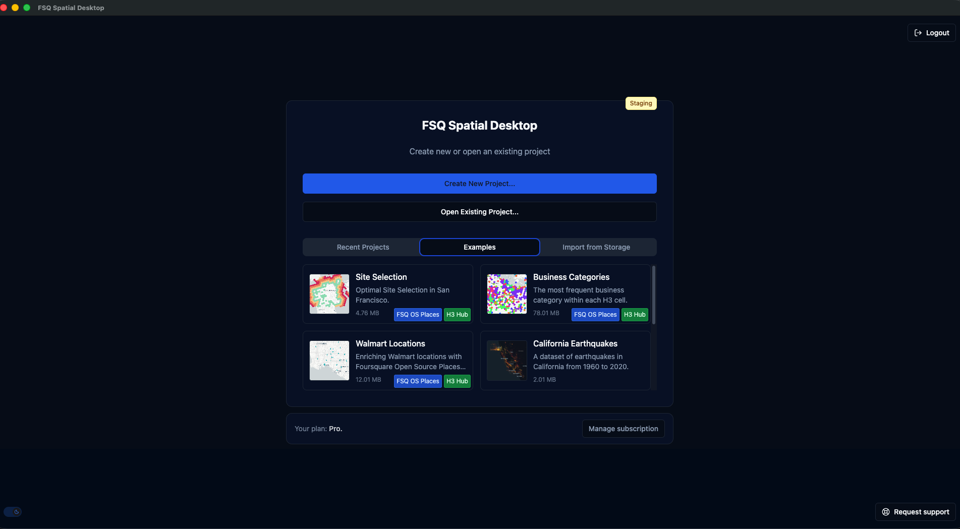
When the application launches, you'll see a welcome screen. Click "Create New Project..."
-
In the "Create and Save New FSQ Spatial Project" dialog box, enter a name for your project in the "Save As" field (e.g., "demo_spatial").
-
Choose the location where you want to save your project file.
-
Click "Save". The application will then initialize the database for your new project.
Add Data to Your Project
To begin your analysis, you need to import your data into the platform from your local or cloud storage:
-
In the FSQ Spatial Desktop interface, click "+ Add Data" in the "Data Sources" panel on the left.
-
In the "Add Data" dialog, select the "Upload" tab.
-
Click "Add files" to browse for your local data files.
-
Navigate to the directory where your data is located, select your data file (e.g., walmart.csv), and click "Open".
-
The selected data will be imported and displayed as a layer on the map.
-
You'll also see it listed under "Tables" in the "Data Sources" panel.
-
To open map layer settings panel click on cogwheel icon (Map settings)
Access FSQ OS Places & H3 Catalog
Add OS Places data
-- read from the s3 bucket directly
CREATE OR REPLACE VIEW os_places AS ( SELECT * FROM read_parquet('s3://fsq-os-places-us-east-1/release/dt=2025-07-08/places/parquet/*.parquet'))
Add the H3 Hub Iceberg Catalog
-- enable access to H3 Hub Iceberg catalog
-- get a token first and paste it in TOKEN
INSTALL iceberg;
INSTALL httpfs;
INSTALL h3 FROM community;
INSTALL spatial;
LOAD httpfs;
CREATE OR REPLACE SECRET iceberg_secret (
   TYPE ICEBERG,
   TOKEN ''
);
ATTACH 'open_h3' AS open_h3 (
   TYPE iceberg,
   SECRET iceberg_secret,
   ENDPOINT 'https://h3-hub-foursquare.acryl.io/gms/iceberg/'
);
SELECT table_schema, table_name FROM information_schema.tables WHERE table_catalog = 'open_h3';
Work with Data & Map Layers
Once your data is added, you can query it and manage its layers. At this point, you can perform the following actions.
-
View Data Columns: In the "Data Sources" panel, expand the imported table (e.g., "walmart") to see its columns (e.g., "lon", "lat", "date").
-
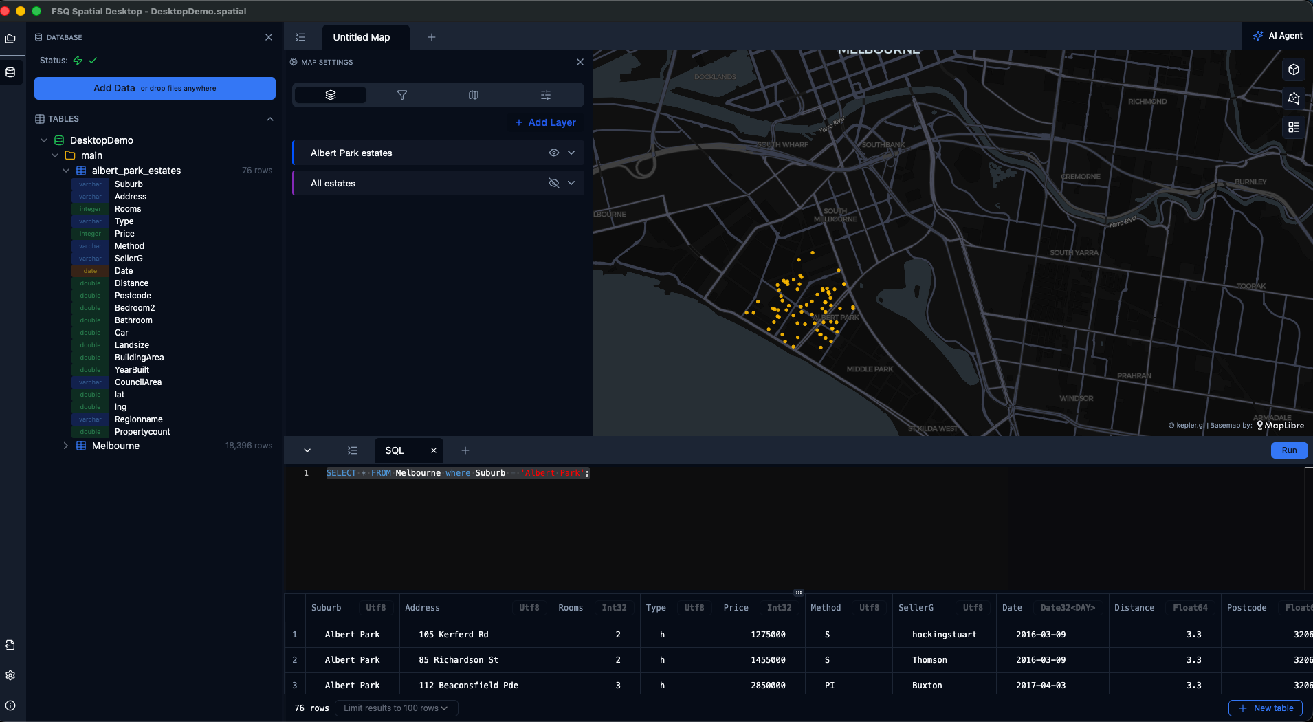
Run SQL Queries: Below the map, you'll find a query editor area labeled "Run" where you can type your SQL query. After entering your query, click the "Run" button (the play icon) to execute it. Any table you create through the query interface will automatically show up in the “Tables” section.
-
Rename Queries: To rename a query, click the down arrow next to the query tab (e.g., "Untitled"), select "Rename", enter a new name (e.g., "FSQ Places", "Enrich"), and then click "Save".
-
Send Data: “+ Add table to map” access this through the table explorer and the three dots expand and push your data to the map.
-
Manage Map Layers: To open the layers panel click on the Map Settings cogwheel button (note that map settings panel is collapsed by default. The "Layers" panel on the right displays the active data layers on your map. From here, you can toggle the visibility of a layer by clicking the eye icon next to its name, delete a layer by clicking the trash can icon, or edit a layer's styling by clicking the pencil icon.
Customize Map Visualization
FSQ Spatial Desktop offers real-time rendering of up to 1 million points with interactive filtering and smooth animations. You can customize how your data is displayed on the map. For instance, you can:
-
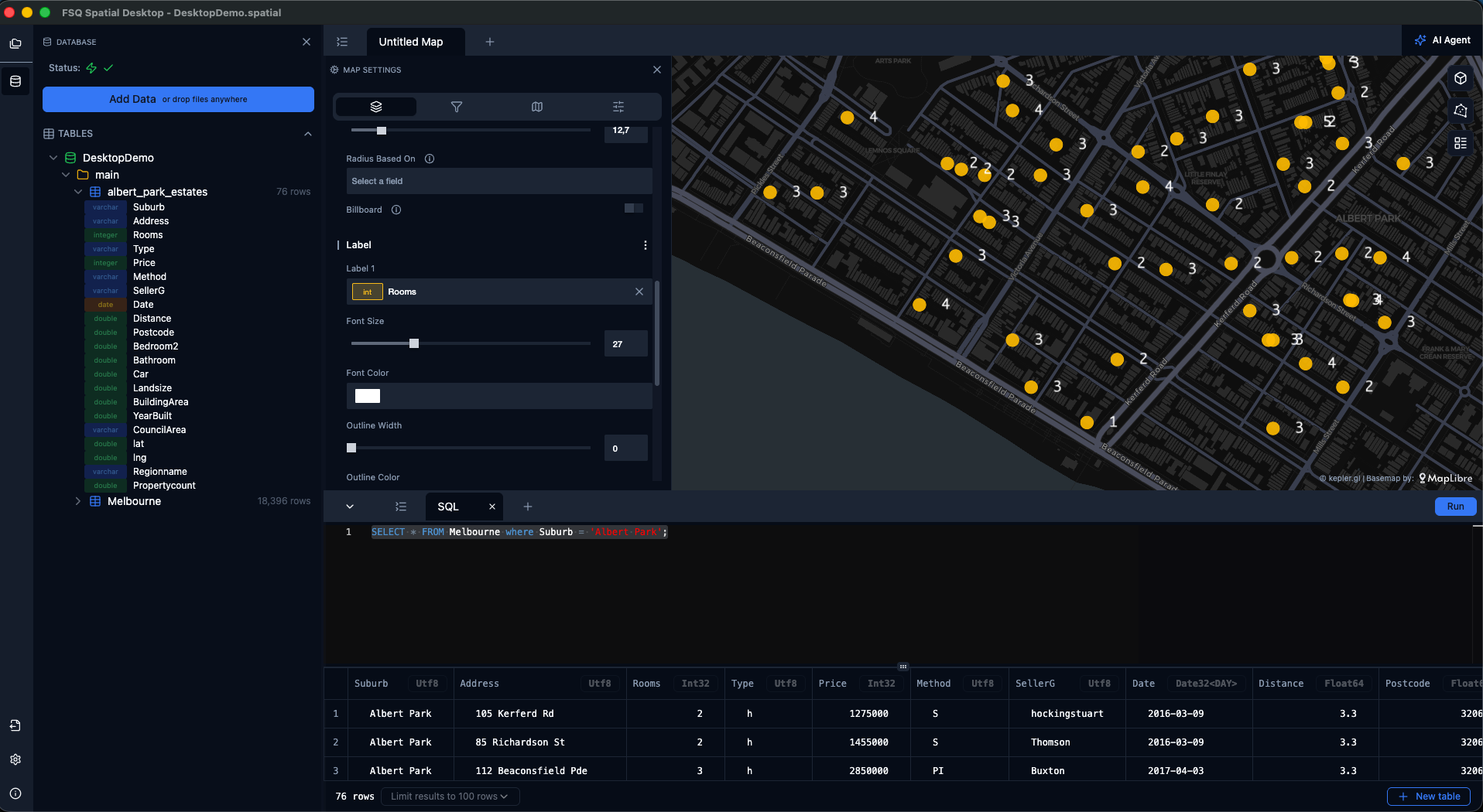
Adjust Point Styling: In the "Layers" panel, click the pencil icon next to a point layer (e.g., "walmart_places"). Under the "Basic" section, you can change the fill color by clicking "Fill Color" and then "Select a field" to color-code points based on a data attribute (e.g., left_name), choosing a color scale from the provided options. Finally, adjust the "Radius" slider to change the size of the points on the map.
-
Change BaseMap Style: To change the base map style, click the "Base Maps" icon in the top left corner of the map window, then select a different base map style from the options (e.g., "Dark Matter", "Satellite With Streets"). This action will change the underlying map imagery.
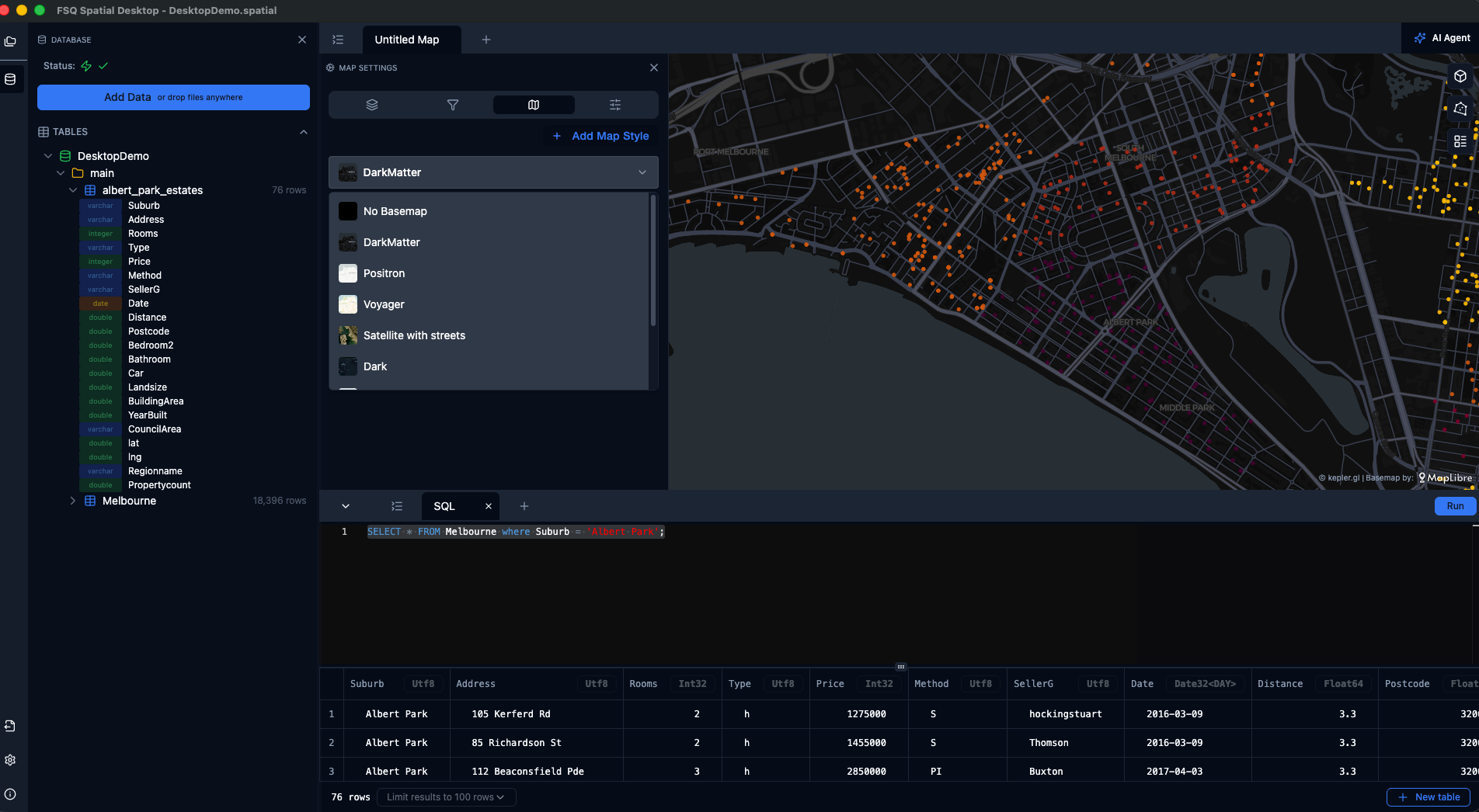
For additional customization options, refer to the documentation on the kepler.gl homepage.
Interact with Map Data
- Pan and Zoom: You can pan the map by clicking and dragging, and zoom in or out by scrolling your mouse wheel.
- Inspect Data Points: Hover over a data point on the map to see a tooltip with its associated information, or click on a data point to display its detailed attributes in the "Interactions" panel on the left.
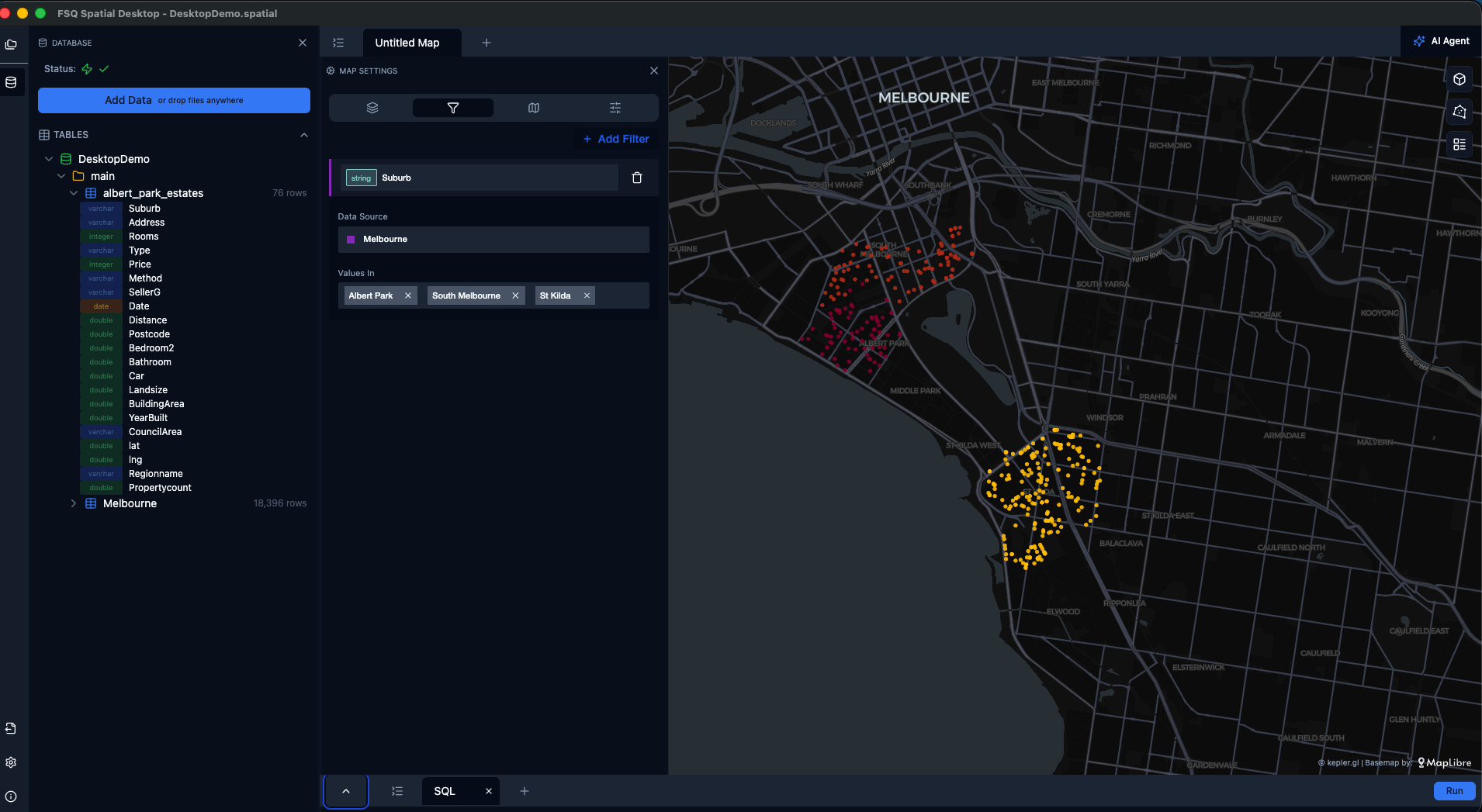
- Filter Data: In the "Filters" panel on the left, click "Add Filter," select the data source and the field you want to filter by (e.g.,
left_name), then enter or select the desired values (e.g.,"Walmart X"). The map will update to show only the filtered data points.
Share a project
How to share a project by email
- Create or open a project.
- Click the Cloud Storage button in the left side menu.(or Menu > File > Cloud Storage).
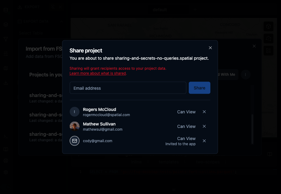
- For the project you want to share, click the three dots button and then click Share.
- Enter emails to share with.
- Click Export.
- Recipients will get an email with a link to open the project in the app.
- Recipients can open the shared project in the app:
- Welcome Screen > Import from Storage > Shared With Me
- Or Cloud Storage > Shared With Me
How to change sharing permissions
- In the app:
- Welcome Screen > Import from Storage > My Projects
- Or Menu > File > Cloud Storage > My Projects
- Find the project and click the Share icon
- Add or remove users to the project as needed
What is shared
-
Shared
- Database file: A copy of your current DuckDB project file (.spatial), created via a DB-level COPY and then uploaded to the storage.
- Datasets added by drag & drop (inserted into DB): Shared as part of the project.
- Tokens/secrets in queries or tables: values you explicitly store in queries or the database are exported (so if you inline them, they will be included). See the Secrets section for details.
- AI queries log / chat: Included with the project by default. You can remove it before sharing if desired.
- Note: Recipients can download the shared project and may re-share it with third parties.
-
Not Shared
- Secrets stored in the Secret Manager are never exported or shared. Only names and descriptions (not values) may appear in exported projects.
- S3 credentials added in the app with S3 browser: Not shared. Each user must add their own credentials via Add Data > S3.
- Local files referenced by path in queries: Not included unless you inserted their contents into the database.
Publish a project
How to publish a project to the oorld
- Go to the Cloud Storage screen where your projects are listed.
- Find the project you want to publish and click the three-dot menu (⋮) on the project card.
- Select Publish from the dropdown menu.
- In the dialog that appears, enter a project name and an optional description for the published version.
- Click Publish. Wait for the process to complete.
- Once published, a Published Project info dialog will appear with shareable links you can copy and send to anyone.
Managing a published project
- To view share links or download stats for an already published project, click the three-dot menu (⋮) and select Publish again. This opens the published project info dialog.
- To unpublish, open the published project info dialog and click Unpublish.
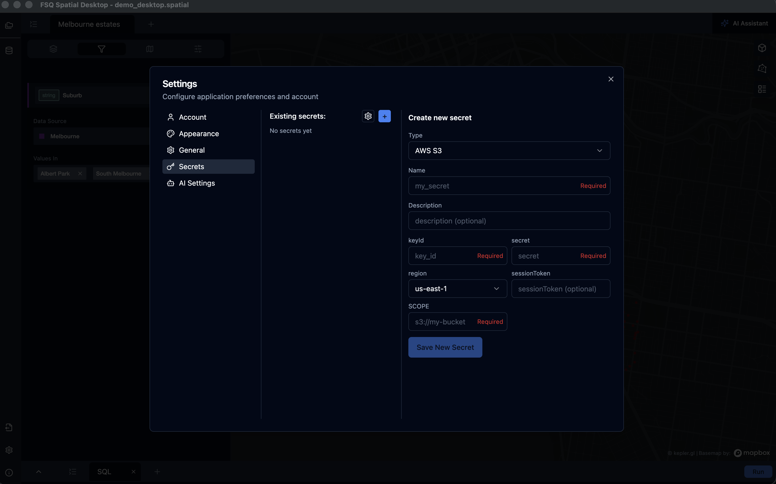
Secrets Manager
Use the Secrets Manager to keep tokens and credentials out of queries so they are not exported or shared with projects. Secrets stored in the Secret Manager are never exported or shared; only their names and descriptions may appear in exported metadata. You can manage secrets through File > Settings > Secrets.
Secrets Manager can inject a value with {{ secrets.name }} but can also add a secret silently to a query when a secret is mentioned with a SECRET name in a query (not only for Iceberg).
Ways to use secrets:
- Secret templates: Reference values with
{{ secrets.token_name }}in SQL queries. The app substitutes them at runtime without writing values to the database.
CREATE OR REPLACE SECRET iceberg_secret (
   TYPE ICEBERG,
   TOKEN {{secrets.iceberg_token}}
);- Named secrets: Define a secret once in Secrets Manager and reference it in SQL queries by name, keeping credentials out of queries.
ATTACH 'open_h3' AS open_h3 (
   TYPE iceberg,
   SECRET secret_name,
   ENDPOINT 'https://h3-hub-foursquare.acryl.io/gms/iceberg/'
);- Automatic detection by protocol and scope: Queries that reference providers by URL scheme or declared scope (e.g., s3://..., gs://...) can use matching secrets from Secrets Manager.
SELECT * FROM 's3://test-project-bucket/points.parquet';Dynamic Tiling
You can transform uploaded datasets into Dynamic Tiles in Spatial Desktop. Dynamic Tile generation allows you to transform massive datasets into an optimized, streamed set of tiles.A dynamic tileset is recommended for large tables to ensure smooth performance by only loading and rendering data tiles that are visible on the current map view.
How to create vector tile dataset
-
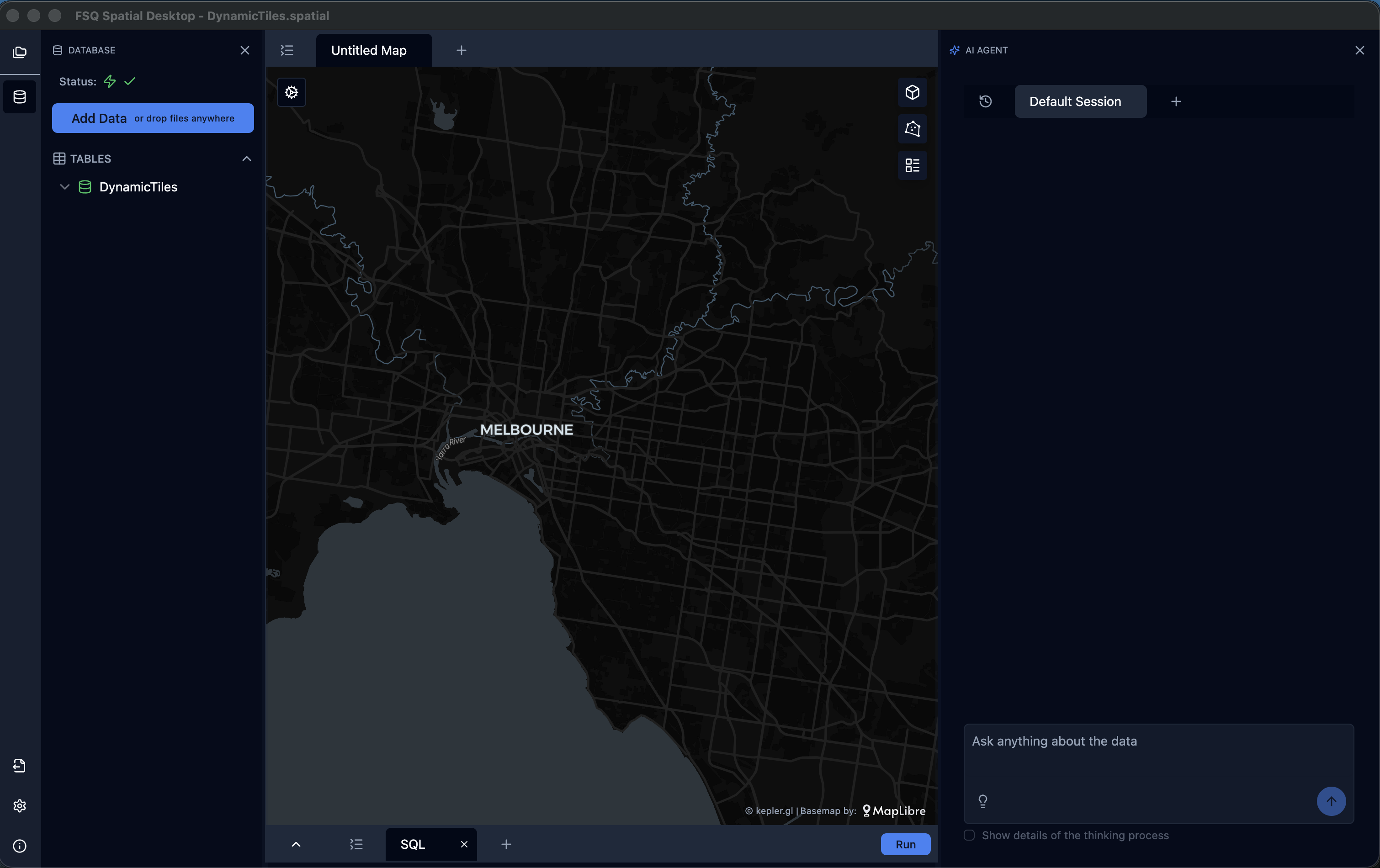
When the dataset is uploaded to Spatial Desktop, open the Database tab and choose Add as Tileset to map option from dataset context menu (i.e. three dots). For datasets that have a big number of rows, tiling will be automatically proposed during the dataset upload.
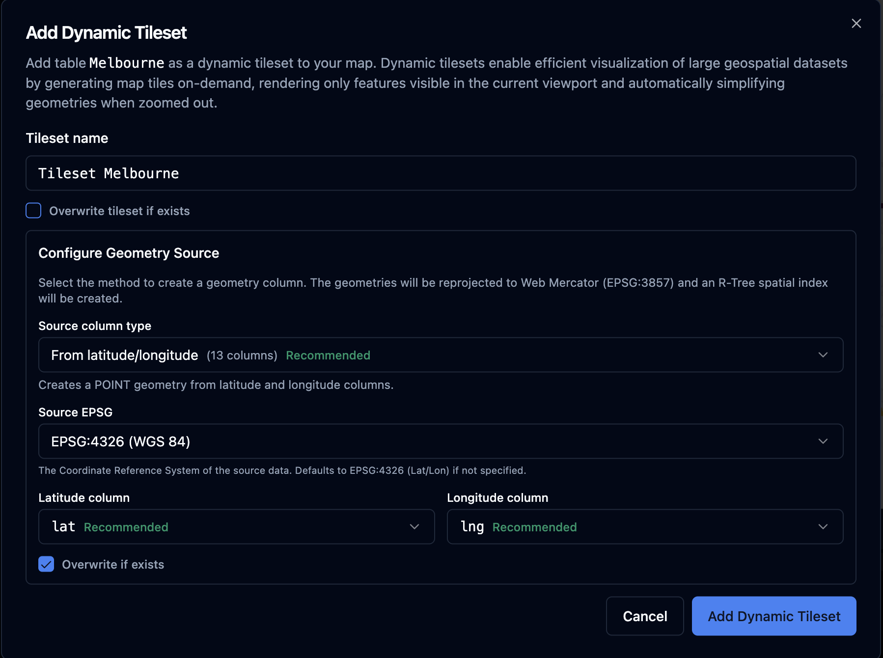
-
In the Dynamic Tileset dialog choose settings based on uploaded dataset. For Source column type choose between: Geometry, latitude/longitude, WKB (BLOB), WKT (string), GeoJSON (string) or H3 cell ID columns based on upload dataset and set Source geometry column. After all options are set correctly click on the “Add Dynamic Tileset” button to add tiled dataset to map.
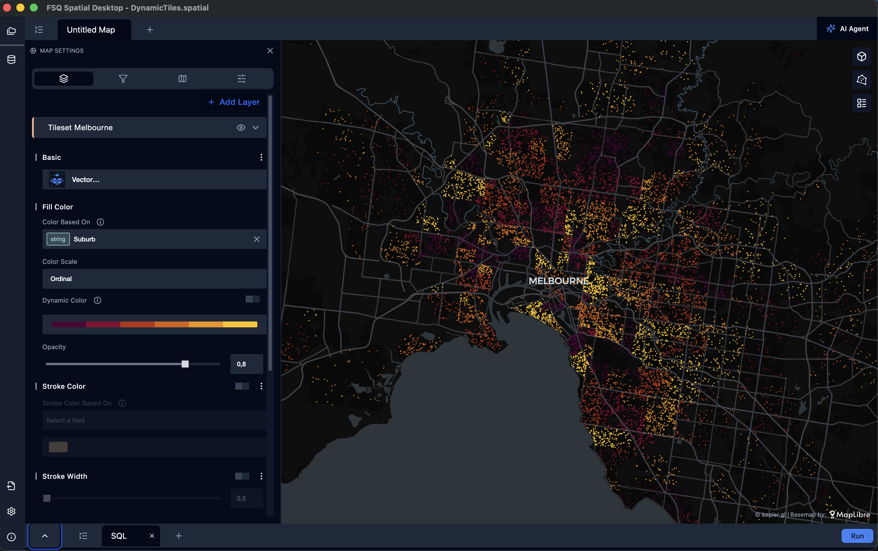
- When tiled data is successfully added to map, go to Layers tab, expand Vector tile layer settings to additionally control layer
Spatial Agent
Spatial Agent is a powerful tool for spatial data analysis using DuckDB. It helps you analyze, visualize, and understand geospatial data through natural language conversations. Simply ask questions about your data, and the assistant will generate SQL queries, create visualizations, and provide insights.
Note: Basic subscription includes $1 worth of tokens as preview, Standard subscriptions include $25 worth of tokens while Pro includes $100 worth of tokens to use towards Spatial Agent. Available tokens can always be checked in the Account card in the Settings window.
It has access to 100M+ Foursquare OS Places POIs over thousands of categories, Foursquare H3 Hub datasets at resolution 8 covering: landuse, population, demographics, crime, health, education, housing, transportation, environment, etc, and administrative boundaries, roads and building footprints data from Overture.
To start using the Spatial Agent, click on the AI agent option in the top right corner..
Core Capabilities
-
Data Querying & Analysis
- Write and execute SQL queries using DuckDB syntax
- Perform complex spatial operations and calculations
- Join, filter, and aggregate data
- Statistical analysis and data exploration
-
Map Visualization
- Create interactive map layers (points, lines, polygons, heatmaps, clusters)
- Visualize H3 hexagons and S2 cells
- Display routes and trip animations
- Support for GeoJSON and various geometry types
-
Chart Creation
- Generate charts using VegaLite (bar charts, line charts, scatter plots, etc.)
- Time series analysis
- Distribution and comparison visualizations
- Interactive tooltips and legends
-
Geospatial Operations
- Geocoding: Convert addresses to coordinates
- Reverse Geocoding: Convert coordinates to addresses
- Routing: Get driving directions between points
- Isochrones: Calculate travel time areas
- Buffer Analysis: Create distance buffers around features
- Spatial Joins: Combine data based on location
-
Administrative Boundaries
- Fetch boundaries for cities, counties, states, countries, ZIP codes
- Analyze data within specific administrative regions
- Get lists of cities within a bounding box
-
Points of Interest (POI)
- Search for places using Foursquare OS Places data
- Find restaurants, hotels, shops, and other venues
- Filter by category and location
-
H3 Hub Integration
- Access global datasets at H3 resolution 8 (city to state level)
- Population, demographics, environmental data, and more
- Combine multiple datasets for advanced analysis
- Note: Explicitly mention "H3 Hub" when you want to use these datasets
-
Road & Building Data
- Fetch road networks for any area
- Get building footprints
- Analyze proximity to infrastructure
How to Use Spatial Agent
- Ask Questions in Natural Language
"Get all pizza places in San Francisco",
"How many starbucks are within 5 minutes drive from my house?",
"Get all roads in San Francisco and create a map based on road types",
"Are ice cream shops always close to pizza stores in New York City?"
-
The Assistant will:
- Understand your request
- Generate appropriate SQL queries
- Execute the queries
- Create visualizations (maps/charts)
- Provide insights and explanations
-
Iterate and Refine
- Ask follow-up questions
- Request different visualizations
- Drill down into specific areas or data points
Data Format Notes:
- Coordinates: Latitude/Longitude in decimal degrees
- Distances: Specify units (meters, kilometers, miles)
- Dates: Various formats supported (YYYY-MM-DD recommended)
- Geometry: WKB format for storage, converted to GEOMETRY for operations
Limitations:
- H3 Hub data is at resolution 8 (best for city to state level, not suitable for country/global analysis)
- Some operations may take time with large datasets (the assistant will notify you)
- Geocoding and routing depend on external services
Getting Help:
- Ask "How do I..." questions for guidance
- Request examples: "Show me an example of..."
- Ask for clarification: "What does this result mean?"
- Request different visualizations: "Can you show this as a chart instead?"
Privacy & Data:
- Your data stays in your local DuckDB database
- Queries are executed locally
- External services used only for geocoding, routing, H3 and LLM models
Updated 5 months ago